Predictability of Distribution
About the function
Predictability of distribution is one of the common methods of determining whether or not two sounds in a language are contrastive or allophonic. The traditional assumption is that two sounds that are predictably distributed (i.e., in complementary distribution) are allophonic, and that any deviation from complete predictability of distribution means that the two sounds are contrastive. [Hall2009], [Hall2012] proposes a way of quantifying predictability of distribution in a gradient fashion, using the information-theoretic quantity of entropy (uncertainty), which is also used for calculating functional load (see Method of calculation), which can be used to document the degree to which sounds are contrastive in a language. This has been shown to be useful in, e.g., documenting sound changes [Hall2013b], understanding the choice of epenthetic vowel in a languages [Hume2013], modeling intra-speaker variability (Thakur 2011), gaining insight into synchronic phonological patterns (Hall & Hall 2013), and understanding the influence of phonological relations on perception ([Hall2009], [Hall2014a]). See also the related measure of Kullback-Leibler divergence (Kullback-Leibler Divergence), which is used in [Peperkamp2006] and applied to acquisition; it is also a measure of the degree to which environments overlap, but the method of calculation differs (especially in terms of environment selection).
It should be noted that predictability of distribution and functional load are not the same thing, despite the fact that both give a measure of phonological contrast using entropy. Two sounds could be entirely unpredictably distributed (perfectly contrastive), and still have either a low or high functional load, depending on how often that contrast is actually used in distinguishing lexical items. Indeed, for any degree of predictability of distribution, the functional load may be either high or low, with the exception of the case where both are 0. That is, if two sounds are entirely predictably distributed, and so have an entropy of 0 in terms of distribution, then by definition they cannot be used to distinguish between any words in the language, and so their functional load, measured in terms of change in entropy upon merger, would also be 0.
Method of calculation
As mentioned above, predictability of distribution is calculated using the same entropy formula as above, repeated here below, but with different inputs.
Entropy:
\(H = -\sum_{i \in N} p_{i} * log_{2}(p_{i})\)
Because predictability of distribution is determined between exactly two sounds, i will have only two values, that is, each of the two sounds. Because of this limitation to two sounds, entropy will range in these situations between 0 and 1. An entropy of 0 means that there is 0 uncertainty about which of the two sounds will occur; i.e., they are perfectly predictably distributed (commonly associated with being allophonic). This will happen when one of the two sounds has a probability of 1 and the other has a probability of 0. On the other hand, an entropy of 1 means that there is complete uncertainty about which of the two sounds will occur; i.e., they are in perfectly overlapping distribution (what might be termed “perfect” contrast). This will happen when each of the two sounds has a probability of 0.5.
Predictability of distribution can be calculated both within an individual environment and across all environments in the language; these two calculations are discussed in turn.
Predictability of Distribution in a Single Environment
For any particular environment (e.g., word-initially; between vowels; before a [+ATR] vowel with any number of intervening consonants; etc.), one can calculate the probability that each of two sounds can occur. This probability can be calculated using either types or tokens, just as was the case with functional load. Consider the following toy data, which is again repeated from the examples of functional load, though just the original distribution of sounds.
| Word | Original | ||
|---|---|---|---|
| Trans. | Type Freq. | Token Freq. | |
| hot | [hɑt] | 1 | 2 |
| song | [sɑŋ] | 1 | 4 |
| hat | [hæt] | 1 | 1 |
| sing | [sɪŋ] | 1 | 6 |
| tot | [tɑt] | 1 | 3 |
| dot | [dɑt] | 1 | 5 |
| hip | [hɪp] | 1 | 2 |
| hid | [hɪd] | 1 | 7 |
| team | [tim] | 1 | 5 |
| deem | [dim] | 1 | 5 |
| toot | [tut] | 1 | 9 |
| dude | [dud] | 1 | 2 |
| hiss | [hɪs] | 1 | 3 |
| his | [hɪz] | 1 | 5 |
| sizzle | [sɪzəl] | 1 | 4 |
| dizzy | [dɪzi] | 1 | 3 |
| tizzy | [tɪzi] | 1 | 4 |
| Total | 17 | 70 | |
Consider the distribution of [h] and [ŋ], word-initially. In this environment, [h] occurs in 6 separate words, with a total token frequency of 20. [ŋ] occurs in 0 words, with, of course, a token frequency of 0. The probability of [h] occurring in this position as compared to [ŋ], then, is 6/6 based on types, or 20/20 based on tokens. The entropy of this pair of sounds in this context, then, is:
\(H_{types/tokens} = -[1 log_{2}(1) + 0 log_{2} (0)] = 0\)
Similar results would obtain for [h] and [ŋ] in word-final position, except of course that it’s [ŋ] and not [h] that can appear in this environment.
For [t] and [d] word-initially, [t] occurs 4 words in this environment, with a total token frequency of 21, and [d] also occurs in 4 words, with a total token frequency of 15. Thus, the probability of [t] in this environment is 4/8, counting types, or 21/36, counting tokens, and the probability of [d] in this environment is 4/8, counting types, or 15/36, counting tokens. The entropy of this pair of sounds is therefore:
\(H_{types} = -[(\frac{4}{8} log_{2}(\frac{4}{8})) + (\frac{4}{8} log_{2}(\frac{4}{8}))] = 1\)
\(H_{types} = -[(\frac{21}{36} log_{2}(\frac{21}{36})) + (\frac{15}{36} log_{2}(\frac{15}{36}))] = 0.98\)
In terms of what environment(s) are interesting to examine, that is of course up to individual researchers. As mentioned in the preface to Predictability of Distribution, these functions are just tools. It would be just as possible to calculate the entropy of [t] and [d] in word-initial environments before [ɑ], separately from word-initial environments before [u]. Or one could calculate the entropy of [t] and [d] that occur anywhere in a word before a bilabial nasal...etc., etc. The choice of environment should be phonologically informed, using all of the resources that have traditionally been used to identify conditioning environments of interest. See also the caveats in the following section that apply when one is calculating systemic entropy across multiple environments.
Predictability of Distribution across All Environments (Systemic Entropy)
While there are times in which knowing the predictability of distribution within a particular environment is helpful, it is generally the case that phonologists are more interested in the relationship between the two sounds as a whole, across all environments. This is achieved by calculating the weighted average entropy across all environments in which at least one of the two sounds occurs.
As with single environments, of course, the selection of environments for the systemic measure need to be phonologically informed. There are two further caveats that need to be made about environment selection when multiple environments are to be considered, however: (1) exhaustivity and (2) uniqueness.
With regard to exhausitivity: In order to calculate the total predictability of distribution of a pair of sounds in a language, one must be careful to include all possible environments in which at least one of the sounds occurs. That is, the total list of environments needs to encompass all words in the corpus that contain either of the two sounds; otherwise, the measure will obviously be incomplete. For example, one would not want to consider just word-initial and word-medial positions for [h] and [ŋ]; although the answer would in fact be correct (they have 0 entropy across these environments), it would be for the wrong reason—i.e., it ignores what happens in word-final position, where they could have had some other distribution.
With regard to uniqueness: In order to get an accurate calculation of the total predictability of distribution of a pair of sounds, it is important to ensure that the set of environments chosen do not overlap with each other, to ensure that individual tokens of the sounds are not being counted multiple times. For example, one would not want to have both [#__] and [__i] in the environment list for [t]/[d] while calculating systemic entropy, because the words team and deem would appear in both environments, and the sounds would (in this case) appear to be “more contrastive” (less predictably distributed) than they might otherwise be, because the contrasting nature of these words would be counted twice.
To be sure, one can calculate the entropy in a set of individual environments that are non-exhaustive and/or overlapping, for comparison of the differences in possible generalizations. But, in order to get an accurate measure of the total predictability of distribution, the set of environments must be both exhaustive and non-overlapping. As will be described below, PCT will by default check whether any set of environments you provide does in fact meet these characteristics, and will throw a warning message if it does not.
It is also possible that there are multiple possible ways of developing a set of exhaustive, non-overlapping environments. For example, “word-initial” vs. “non-word-initial” would suffice, but so would “word-initial” vs. “word-medial” vs. “word-final.” Again, it is up to individual researchers to determine which set of environments makes the most sense for the particular pheonmenon they are interested in. See [Hall2012] for a comparison of two different sets of possible environments in the description of Canadian Raising.
Once a set of exhaustive and non-overlapping environments has been determined, the entropy in each individual environment is calculated, as described in Predictability of Distribution in a Single Environment. The frequency of each environment itself is then calculated by examining how many instances of the two sounds occurred in each environment, as compared to all other environments, and the entropy of each environment is weighted by its frequency. These frequency-weighted entropies are then summed to give the total average entropy of the sounds across the environments. Again, this value will range between 0 (complete predictability; no uncertainty) and 1 (complete unpredictability; maximal uncertainty). This formula is given below; e represents each individual environment in the exhaustive set of non-overlapping environments.
Formula for systemic entropy:
\(H_{total} = -\sum_{e \in E} H(e) * p(e)\)
As an example, consider [t]/[d]. One possible set of exhaustive, non-overlapping environments for this pair of sounds is (1) word-initial and (2) word-final. The relevant words for each environment are shown in the table below, along with the calculation of systemic entropy from these environments.
The calculations for the entropy of word-initial environments were given above; the calculations for word-final environments are analogous.
To calculate the probability of the environments, we simply count up the number of total words (either types or tokens) that occur in each environment, and divide by the total number of words (types or tokens) that occur in all environments.
Calculation of systemic entropy of [t] and [d]:
| e | [t]- words |
[d]- words |
Types | Types | ||||
|---|---|---|---|---|---|---|---|---|
| H(e) | p(e) | p(e) * H(e) | H(e) | p(e) | p(e) * H(e) | |||
| [#__] | tot, team, toot, tizzy | dot, dude, deem, dizzy | 1 | (4+4)/ (8+7) =8/15 | 0.533 | 0.98 | (21+15)/ (36+29) =36/65 | 0.543 |
| [__#] | hot, hat, tot, dot, toot | hid, dude | 0.863 | 7/15 | 0.403 | 0.894 | 29/65 | 0.399 |
| 0.533+0.403=0.936 | 0.543+0.399=0.942 | |||||||
In this case, [t]/[d] are relatively highly unpredictably distributed (contrastive) in both environments, and both environments contributed approximately equally to the overall measure. Compare this to the example of [s]/[z], shown below.
Calculation of systemic entropy of [s] and [z]:
| e | [s]- words |
[z]- words |
Types | Types | ||||
|---|---|---|---|---|---|---|---|---|
| H(e) | p(e) | p(e) * H(e) | H(e) | p(e) | p(e) * H(e) | |||
| [#__] | song, sing, sizzle | 0 | 3/8 | 0 | 0 | 14/33 | 0 | |
| [__#] | hiss | his | 1 | 2/8 | 0.25 | 0.954 | 8/33 | 0.231 |
| [V_V] | sizzle, dizzy, tizzy | 0 | 3/8 | 0 | 0 | 11/33 | 0 | |
| 0.25 | 0.231 | |||||||
In this case, there is what would traditionally be called a contrast word finally, with the minimal pair hiss vs. his; this contrast is neutralized (made predictable) in both word-initial position, where [s] occurs but [z] does not, and intervocalic position, where [z] occurs but [s] does not. The three environments are roughly equally probable, though the environment of contrast is somewhat less frequent than the environments of neutralization. The overall entropy of the pair of sounds is on around 0.25, clearly much closer to perfect predictability (0 entropy) than [t]/[d].
Note, of course, that this is an entirely fictitious example—that is, although these are real English words, one would not want to infer anything about the actual relationship between either [t]/[d] or [s]/[z] on the basis of such a small corpus. These examples are simplified for the sake of illustrating the mathematical formulas!
“Predictability of Distribution” Across All Environments (i.e., Frequency-Only Entropy)
Given that the calculation of predictability of distribution is based on probabilities of occurrence across different environments, it is also possible to calculate the overall entropy of two segments using their raw probabilities and ignoring specific environments. Note that this doesn’t really reveal anything about predictability of distribution per se; it simply gives the uncertainty of occurrence of two segments that is related to their relative frequencies. This is calculated by simply taking the number of occurrences of each of sound 1 (N1) and sound 2 (N2) in the corpus as a whole, and then applying the following formula:
Formula for frequency-only entropy:
\(H = (-1) * [(\frac{N1}{N1+N2}) log_{2} (\frac{N1}{N1+N2}) +(\frac{N2}{N1+N2}) log_{2} (\frac{N2}{N1+N2})]\)
The entropy will be 0 if one or both of the sounds never occur(s) in the corpus. The entropy will be 1 if the two sounds occur with exactly the same frequency. It will be a number between 0 and 1 if both sounds occur, but not with the same frequency.
Note that an entropy of 1 in this case, which was analogous to perfect contrast in the environment-specific implementation of this function, does not align with contrast here. For example, [h] and [ŋ] in English, which are in complementary distribution, could theoretically have an entropy of 1 if environments are ignored and they happened to occur with exactly the same frequency in some corpus. Similarly, two sounds that do in fact occur in the same environments might have a low entropy, close to 0, if one of the sounds is vastly more frequent than the other. That is, this calculation is based ONLY on the frequency of occurrence, and not actually on the distribution of the sounds in the corpus. This function is thus useful only for getting a sense of the frequency balance / imbalance between two sounds. Note that one can also get total frequency counts for any segment in the corpus through the “Summary” information feature (Summary information about a corpus).
Implementing the predictability of distribution function in the GUI
Assuming a corpus has been opened or created, predictability of distribution is calculated using the following steps.
- Getting started: Choose “Analysis” / “Calculate predictability of distribution...” from the top menu bar.
- Sound selection: On the left-hand side of the “Predictability of distribution” dialogue box, select the two sounds of interest by clicking “Add pair of sounds. The order of the sounds is irrelevant; picking [i] first and [u] second will yield the same results as [u] first and [i] second. Currently, PCT only allows entire segments to be selected; the next release will allow a “sound” to be defined as a collection of feature values. The segment choices that are available will automatically correspond to all of the unique transcribed characters in your corpus. You can select more than one pair of sounds to examine in the same environments; each pair of sounds will be treated individually.
- Environments: Click on “Add environment” to add an environment in
which to calculate predictability of distribution. The left side of
the “Create environment” dialogue box allows left-hand environments
to be specified (e.g., [+back]___), while the right side allows
right-hand environments to be specified (e.g., __#). Both can be used
simultaneously to specify environments on both sides (e.g., [+back]__#).
- Basis for building environments (segments vs. features): Environments can be selected either as entire segments (including #) or as bundles of features. Select from the drop-down menu which you prefer. Each side of an environment can be specified using either type.
- Segment selection: To specify an environment using segments, simply click on the segment desired.
- Feature selection: To specify an environment using features, select the first feature from the list (e.g., [voice]), and then specify whether you want it to be [+voice] or [-voice] by selecting “Add [+feature]” or “Add [-feature]” as relevant. To add another feature to this same environment, select another feature and again add either the + or – value.
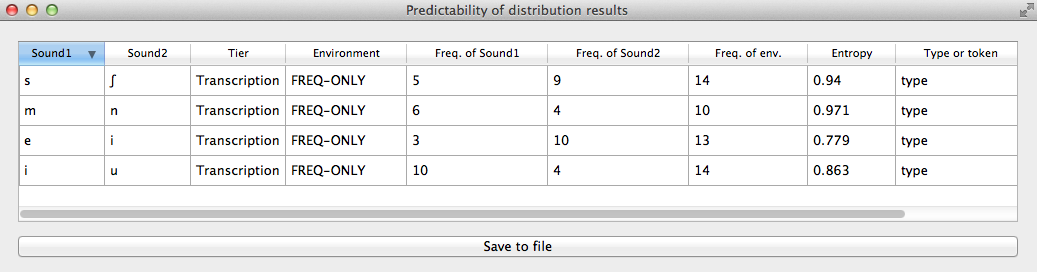
- No environments: Note that if NO environments are added, PCT will calculate the overall predictability of distribution of the two sounds based only on their frequency of occurrence. This will simply count the frequency of each sound in the pair and calculate the entropy based on those frequencies (either type or token). See below for an example of calculating environment-free entropy for four different pairs in the sample corpus:
- Environment list: Once all features / segments for a given environment have been selected, for both the left- and right-hand sides, click on “Add”; it will appear back in the “Predictability of Distribution” dialogue box in the environment list. To automatically return to the environment selection window to select another environment, click on “Add and select another” instead. Individual environments from the list can be selected and removed if it is determined that an environment needs to be changed. It is this list that PCT will verify as being both exhaustive and unique; i.e., the default is that the environments on this list will exhaustively cover all instances in your corpus of the selected sounds, but will do so in such a way that each instance is counted exactly once.
- Analysis tier: Under “Options,” first pick the tier on which you want predictability of distribution to be calculated. The default is for the entire transcription to be used, such that environments are defined on any surrounding segments. If a separate tier has been created as part of the corpus (see Creating new tiers in the corpus), however, predictability of distribution can be calculated on this tier. For example, one could extract a separate tier that contains only vowels, and then calculate predictability of distribution based on this tier. This makes it much easier to define non-adjacent contexts. For instance, if one wanted to investigate the extent to which [i] and [u] are predictably distributed before front vs. back vowels, it will be much easier to to specify that the relevant environments are __[+back] and __[-back] on the vowel tier than to try to account for possible intervening segments on the entire transcription tier.
- Type vs. Token Frequency: Next, pick whether you want the calculation to be done on types or tokens, assuming that token frequencies are available in your corpus. If they are not, this option will not be available. (Note: if you think your corpus does include token frequencies, but this option seems to be unavailable, see Required format of corpus on the required format for a corpus.)
- Exhaustivity & Uniqueness: The default is for PCT to check for both
exhaustivity and uniqueness of environments, as described above in
Predictability of Distribution across All Environments (Systemic Entropy). Un-checking this box will turn off this mechanism. For
example, if you wanted to compare a series of different possible
environments, to see how the entropy calculations differ under
different generalizations, uniqueness might not be a concern. Keep
in mind that if uniqueness and exhaustivity are not met, however,
the calculation of systemic entropy will be inaccurate.
- If you ask PCT to check for exhaustivity, and it is not met, an error message will appear that warns you that the environments you have selected do not exhaustively cover all instances of the symbols in the corpus, as in the following; the “Show details...” option has been clicked to reveal the specific words that occur in the corpus that are not currently covered by your list of environments. Furthermore, a .txt file is automatically created that lists all of the words, so that the environments can be easily adjusted. This file is stored in the ERRORS folder within the working directory that contains the PCT software, and can be accessed directly by clicking “Open errors directory.” If exhaustivity is not important, and only the entropy in individual environments matters, then it is safe to not enforce exhaustivity; it should be noted that the weighted average entropy across environments will NOT be accurate in this scenario, because not all words have been included.

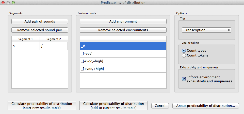
Here’s an example of correctly exhaustive and unique selections for calculating the predictability of distribution based on token frequency for [s] and [ʃ] in the sample corpus:
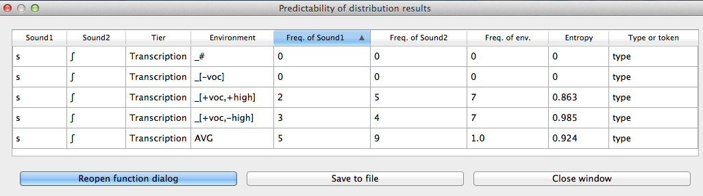
- Entropy calculation / results: Once all environments have been specified, click “Calculate predictability of distribution.” If you want to start a new results table, click that button; if you’ve already done at least one calculation and want to add new calculations to the same table, select the button with “add to current results table.” Results will appear in a pop-up window on screen. The last row for each pair gives the weighted average entropy across all selected environments, with the environments being weighted by their own frequency of occurrence. See the following example:
- Output file / Saving results: If you want to save the table of results, click on “Save to file” at the bottom of the table. This opens up a system dialogue box where the directory and name can be selected.
To return to the function dialogue box with your most recently used selections, click on “Reopen function dialog.” Otherwise, the results table can be closed and you will be returned to your corpus view.