Mutual Information
About the function
Mutual information 1 is a measure of how much dependency there is between two random variables, X and Y. That is, there is a certain amount of information gained by learning that X is present and also a certain amount of information gained by learning that Y is present. But knowing that X is present might also tell you something about the likelihood of Y being present, and vice versa. If X and Y always co-occur, then knowing that one is present already tells you that the other must also be present. On the other hand, if X and Y are entirely independent, then knowing that one is present tells you nothing about the likelihood that the other is present.
In phonology, there are two primary ways in which one could interpret X and Y as random variables. In one version, which we will call word-internal co-occurrence pointwise mutual information, X and Y are equivalent random variables, each varying over “possible speech sounds in some unit” (where the unit could be any level of representation, e.g. a word or even a non-meaningful unit such as a bigram). In this case, one is measuring how much the presence of X anywhere in the defined unit affects the presence of Y in that same unit, regardless of the order in which X and Y occur, such that the mutual information of (X; Y) is the same as the mutual information of (Y; X), and furthermore, the pointwise mutual information of any individual value of each variable (X = a; Y = b) is the same as the pointwise mutual information of (X = b; Y = a). Although this is perhaps the most intuitive version of mutual information, given that it does give a symmetric measure for “how much information does the presence of a provide about the presence of b,” we are not currently aware of any work that has attempted to use this interpretation of MI for phonological purposes.
The other interpretation of MI, which we will call ordered pair pMI, assumes that X and Y are different random variables, with X being “possible speech sounds occurring as the first member of a bigram” and Y being “possible speech sounds occurring as the second member of a bigram.” This gives a directional interpretation to mutual information, such that, while the mutual information of (X; Y) is the same as the mutual information of (Y; X), the pointwise mutual information of (X = a; Y = b) is NOT the same as the pointwise mutual information of (X = b; Y = a), because the possible values for X and Y are different. (It is still, trivially, the case that the pointwise mutual information of (X = a; Y = b) and (Y = b; X = a) are equal.)
This latter version of mutual information has primarily been used as a measure of co-occurrence restrictions (harmony, phonotactics, etc.). For example, [Goldsmith2012] use pointwise mutual information as a way of examining Finnish vowel harmony; see also discussion in [Goldsmith2002]. Mutual information has also been used instead of Transitional Probability as a way of finding boundaries between words in running speech, with the idea that bigrams that cross word boundaries will have, on average, lower values of mutual information than bigrams that are within words (see [Brent1999], [Rytting2004]). Note, however, that in order for this latter use of mutual information to be useful, one must be using a corpus based on running text rather than a corpus that is simply a list of individual words and their token frequencies.
Note that pointwise mutual information can also be expressed in terms of the information content of each of the members of the bigram. Information is measured as the negative log of the probability of a unit \((I(a) = -log_2*p(a))\), so the pMI of a bigram ab is also equal to \(I(a) + I(b) – I(ab)\).
Method of calculation
Both of the interpretations of mutual information described above are implemented in PCT. We refer to the first one, in which X and Y are interpreted as equal random variables, varying over “possible speech sounds in a unit,” as word-internal co-occurrence pointwise mutual information (pMI), because we specifically use the word as the unit in which to measure pMI. We refer to the second one, in which X and Y are different random variables, over either the first or second members of bigrams, as ordered pair pMI.
The general formula for all versions of pointwise mutual information is given below; it is the binary logarithm of the joint probability of X = a and Y = b, divided by the product of the individual probabilities that X = a and Y = b.
\(pMI = log_2 (\frac{p(X=a \& Y = b)}{p(X=a)*p(Y=b)})\)
Note that in PCT, calculations are not rounded until the final stage, whereas in [Goldsmith2012], rounding was done at some intermediate stages as well, which may result in slightly different final pMI values being calculated.
Word-internal co-occurrence pMI
In this implementation of pMI, the joint probability that X = a and Y = b is equal to the probability that some unit (in our case, a word) contains both a and b in any order. Therefore, the pMI of the sounds a and b is equal to the binary logarithm of the probability of some word containing both a and b, divided by the product of the individual probabilities of a word containing a and a word containing b.
Pointwise mutual information for individual segments:
\(pMI_{word-internal} = log_2 (\frac{p(a \in W \& b \in W)} {p(a \in W)*p(b \in W)})\)
Ordered pair pMI
In this version of pMI, the joint probability that X = a and Y = b is equal to the probability of occurrence of the sequence ab. Therefore, the pointwise mutual information of a bigram (e.g., ab) is equal to the binary logarithm of the probability of the bigram divided by the product of the individual segment probabilities, as shown in the formula below.
Pointwise mutual information for bigrams:
\(pMI_{ordered-pair} = log_2 (\frac{p(ab)} {p(a)*p(b)})\)
For example, given the bigram [a, b], its pointwise mutual information is the binary logarithm of the probability of the sequence [ab] in the corpus divided by a quantity equal to the probability of [a] times the probability of [b]. Bigram probabilities are calculated by dividing counts by the total number of bigrams, and unigram probabilities are calculated equivalently.
Environment filters
In addition to simply calculating mutual information based on any occurrence of the two segments, the user may limit the occurrences that “count” as occurrences of those segments by specific environments using Environment Selection. For example, one might be interested in calculating the ordered pair pMI not in all positions but only in word-final positions (environment filtering is irrelevant for word-internal co-occurrence pMI). Let’s assume we calculate pMI of the bigram [ʃ,i] in the mini corpus below. For the purpose of presentation, each word occurs once in the corpus and transcriptions contain word boundaries (#) on both sides, contra the default setting for word boundaries. In this table, we will include both word boundaries as potential elements of bigrams (e.g. in this table, the word [#ʃi#] contains three bigrams, [#ʃ], [ʃi], and [i#]), though we will subsequently discuss other options. See step 6 of “Calculating mutual information in the GUI” (Word boundary count) for general information.
Word |
Trans. |
Freq. |
Num. seg. |
Num. bigram |
Num. [ʃ] |
Num. [i] |
Num. [ʃi] |
|---|---|---|---|---|---|---|---|
ʃaʃi |
[#ʃaʃi#] |
1 |
6 |
5 |
2 |
1 |
1 |
ʃi |
[#ʃi#] |
1 |
4 |
3 |
1 |
1 |
1 |
ʃisota |
[#ʃisota#] |
1 |
8 |
7 |
1 |
1 |
1 |
i |
[#i#] |
1 |
3 |
2 |
0 |
1 |
0 |
Total |
4 |
21 |
17 |
4 |
4 |
3 |
|
One can calculate pMI of the bigram [ʃ,i] in this corpus with or without environment filtering.
Let’s first calculate pMI(ʃ,i) without environment filtering as the baseline. Using the numbers presented in the table,
\(pMI (ʃ,i) = log_2 (\frac{p(ʃi)} {p(ʃ)*p(i)}) = 2.28\)
since, \(p(ʃi) = \frac{3}{17}\), \(p(ʃ) = \frac{4}{21}\), and \(p(i) = \frac{4}{21}\)
Meanwhile, when calculating pMI for the same bigram only in word-final position, i.e., in the context [__#], we “clip” or “filter” the corpus, leaving only the last two segment positions in each word for potential bigrams. (Note that the location of the potential bigrams is dependent on the Environment Selection. For example, calculating the same bigram in a word-initial position would require leaving the first two positions.) In the two tables below, the result of clipping is shown in the column labeled “Context”. In this case, we have simply extracted all bigrams that occur in the context __#.
When applying environment filters, the question of word boundaries takes on an additional complication. Specifically, we must decide whether a word boundary is allowed to count as part of a bigram (separately from the presence of the word boundary that happens to be a part of our selected context in this case). Whether the word boundary can be a part of potential bigram is critical for the last word, [#i#]. If # can count as a member of a bigram, the word has the bigram [#i] in the context [__#]. If # is NOT allowed to count a a member of a bigram, then the only segment in the context [__#] in this word is not a bigram (it’s the single segment [i]), and so the word [#i#] is ignored entirely.
The comparison between including or excluding # in bigrams is presented in the two tables below. Note how the “Context” columns are different in the row for [#i#].
Word boundary counts as a member of a bigram
Word |
Trans. |
Context |
Freq. |
Num. seg. |
Num. bigram |
Num. [ʃ] |
Num. [i] |
Num. [ʃi] |
|---|---|---|---|---|---|---|---|---|
ʃaʃi |
[#ʃaʃi#] |
[ʃi#] |
1 |
3 |
2 |
1 |
1 |
1 |
ʃi |
[#ʃi#] |
[ʃi#] |
1 |
3 |
2 |
1 |
1 |
1 |
ʃisota |
[#ʃisota#] |
[ta#] |
1 |
3 |
2 |
0 |
0 |
0 |
i |
[#i#] |
[#i#] |
1 |
3 |
2 |
0 |
1 |
0 |
Total |
4 |
12 |
8 |
2 |
3 |
2 |
||
Now, we can calculate pMI(ʃ,i) in this “Clipped corpus,” that is, using the forms in the “Context” column.
\(pMI_{(\_\#, WB\ bigram)} (ʃ,i) = log_2 (\frac{p(ʃi)} {p(ʃ)*p(i)}) = 2.58\)
since, \(p(ʃi) = \frac{2}{8}\), \(p(ʃ) = \frac{2}{12}\), and \(p(i) = \frac{3}{12}\)
Word boundary does NOT count as a member of a bigram
Word |
Trans. |
Context |
Freq. |
Num. seg. |
Num. bigram |
Num. [ʃ] |
Num. [i] |
Num. [ʃi] |
|---|---|---|---|---|---|---|---|---|
ʃaʃi |
[#ʃaʃi#] |
[ʃi#] |
1 |
3 |
2 |
1 |
1 |
1 |
ʃi |
[#ʃi#] |
[ʃi#] |
1 |
3 |
2 |
1 |
1 |
1 |
ʃisota |
[#ʃisota#] |
[ta#] |
1 |
3 |
2 |
0 |
0 |
0 |
i |
[#i#] |
N/A |
||||||
Total |
3 |
9 |
6 |
2 |
2 |
2 |
||
Again, we can calculate pMI(ʃ,i) in this “Clipped corpus,” that is, using the forms in the “Context” column. Note that the word [#i#] does not have the context since the word-initial word boundary symbol cannot be a part of bigram.
\(pMI_{(\_\#)} (ʃ,i) = log_2 (\frac{p(ʃi)} {p(ʃ)*p(i)}) = 2.75\)
since, \(p(ʃi) = \frac{2}{6}\), \(p(ʃ) = \frac{2}{9}\), and \(p(i) = \frac{2}{9}\)
Calculating mutual information in the GUI
To start the analysis, click on “Analysis” / “Calculate mutual information…” in the main menu. The choice between the two algorithms depends on the setting of Set domain to word. The default is ordered pair pMI and choosing “set domain to word” switches to the unordered word-internal co-occurrence pMI. Note that switching to word-internal pMI is not available when the environment filter is on.
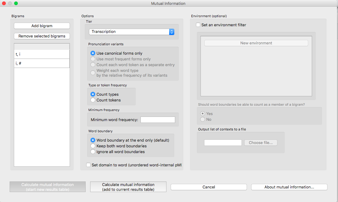
Follow these steps to calculate mutual information:
Bigrams: Click on the “Add bigram” button in the “Mutual Information” dialogue box to get the bigram_selector dialogue box. Note that the order of the sounds matters if “Set domain to word (unordered word-internal pMI)” is unchecked (the default).
Tier: Mutual information can be calculated on any available tier. The default is transcription. If a vowel tier has been created, for example, one could calculate the mutual information between vowels on that tier, ignoring intervening consonants, to examine harmony effects.
Pronunciation variants: If the corpus contains multiple pronunciation variants for lexical items, select what strategy should be used. For details, see Pronunciation Variants.
Type vs. Token Frequency: Next, pick whether you want the calculation to be done on types or tokens, assuming that token frequencies are available in your corpus. If they are not, this option will not be available. (Note: if you think your corpus does include token frequencies, but this option seems to be unavailable, see Required format of corpus on the required format for a corpus.)
Minimum frequency: It is possible to set a minimum token frequency for words in the corpus to be included in the calculation. This allows easy exclusion of rare words. To include all words in the corpus, regardless of their token frequency, leave the slot empty or set it to 0. Note that if a minimum frequency set, all words below that frequency are simply ignored entirely for the purposes of the calculation.
Word boundary count: Select an option for word boundary. The default is to assume that there is only one boundary per word, and that it is in final position (as is assumed in [Goldsmith2012]). This is based on the assumption that in running text, the final boundary of word 1 will be the initial boundary of word 2, so that there is no need to have two boundaries per word. Select “Keep both word boundaries” to have boundaries on both sides, or “Ignore all word boundaries” to ignore all word boundaries in the calculation. Note that this is a separate issue from whether word boundaries should be considered part of a bigram when an environment filter is applied (see step 8 below).
Set domain to word (unordered word-internal pMI): Select this button to calculate Word-internal co-occurrence pMI. Note that environment filtering is not meaningful in unordered word-internal pMI.
Environment (optional): Select “Set an environment filter” button to add environment filters. (see Environment filters for how environment filtering works in calculating pMI, and Environment Selection for how to add an environment)
Should word boundaries be able to count as a member of a bigram?: As described in Environment filters, the user can include or exclude word boundaries as a member of a potential bigram.
Output list of contexts to a file: One can provide a path to export the corpus ‘context’, i.e., the result of environment filtering that is to be fed into calculating pMI. The exported file can be found at the specified location after clicking “Calculate mutual information.”
Results: Once all options have been selected, click “Calculate mutual information.” If this is not the first calculation, and you want to add the results to a pre-existing results table, select the choice that says “add to current results table.” Otherwise, select “start new results table.” A dialogue box will open, showing a table of the results. The mutual information value is located on the right-most column. The table also includes machine-provided information such as corpus name and PCT version, as well as options selected by the user such as first segment, second segment, domain (i.e., which one of the two algorithms), the word boundary option, the tier used, frequency type, pronunciation variants, minimum word frequency and environment. To save these results to a .txt file, click on “Save to file” at the bottom of the table.
The following image shows the inventory window used for selecting bigrams in the sample corpus:
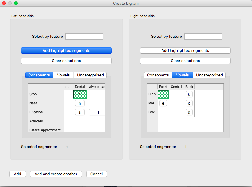
The selected bigrams appear in the list in the “Mutual Information” dialogue box. You will see that we added another bigram, [i, #]. We did this by clicking Add and create another after entering the bigram [t,i], selecting i and # from the inventory chart. # (the word boundary symbol) should be under Uncategorized:
The resulting mutual information results table:
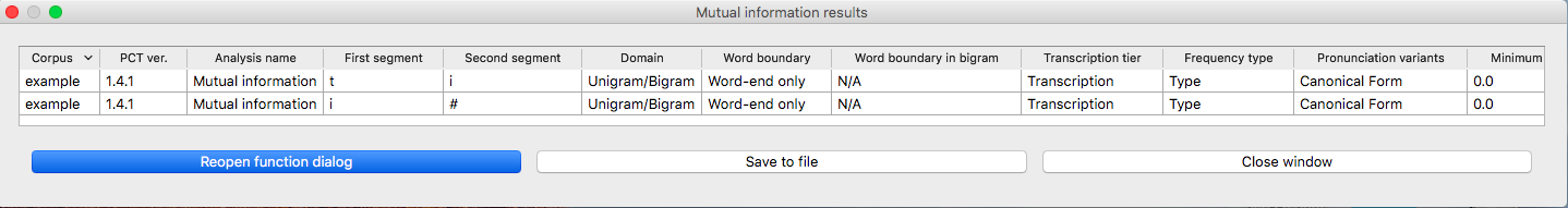
To return to the function dialogue box with your most recently used selections, click on “Reopen function dialog.” Otherwise, the results table can be closed and you will be returned to your corpus view.
Implementing the mutual information function on the command line
In order to perform this analysis on the command line, you must enter a command in the following format into your Terminal:
pct_mutualinfo CORPUSFILE [additional arguments]
…where CORPUSFILE is the name of your *.corpus file. If not calculating
the mutal informations of all bigrams (using -l), the query bigram must
be specified using -q, as -q QUERY. The bigram QUERY must
be in the format s1,s2 where s1 and s2 are the first and second
segments in the bigram. You may also use command line options to
change the sequency type to use for your calculations, or to specify
an output file name. Descriptions of these arguments can be viewed by
running pct_mutualinfo -h or pct_mutualinfo --help. The help text
from this command is copied below, augmented with specifications of
default values:
Positional arguments:
- corpus_file_name
Name of corpus file
Mandatory argument group (call must have one of these two):
Optional arguments:
- -c CONTEXT_TYPE
- --context_type CONTEXT_TYPE
How to deal with variable pronunciations. Options are ‘Canonical’, ‘MostFrequent’, ‘SeparatedTokens’, or ‘Weighted’. See documentation for details.
- -s SEQUENCE_TYPE
- --sequence_type SEQUENCE_TYPE
The attribute of Words to calculate MI over. Normally, this will be the transcription, but it can also be the spelling or a user-specified tier.
EXAMPLE 1: If your corpus file is example.corpus (no pronunciation variants) and you want to calculate the mutual information of the bigram ‘si’ using defaults for all optional arguments, you would run the following command in your terminal window:
pct_mutualinfo example.corpus -q s,i
EXAMPLE 2: Suppose you want to calculate the mutual information of the bigram ‘si’ on the spelling tier. In addition, you want the script to produce an output file called output.txt. You would need to run the following command:
pct_mutualinfo example.corpus -q s,i -s spelling -o output.txt
EXAMPLE 3: Suppose you want to calculate the mutual information of all bigram types in the corpus. In addition, you want the script to produce an output file called output.txt. You would need to run the following command:
pct_mutualinfo example.corpus -l -o output.txt
Classes and functions
For further details about the relevant classes and functions in PCT’s source code, please refer to Mutual information.
- 1
The algorithm in PCT calculates what is sometimes referred to as the “pointwise” mutual information of a pair of units X and Y, in contrast to “mutual information,” which would be the expected average value of the pointwise mutual information of all possible values of X and Y. We simplify to use “mutual information” throughout.